PROCESS

Architecture starts long before form, and keeps changing after it appears.

The sequence is intended to clarify how the work develops: first by reading existing conditions, then by organizing space through geometry, testing critical decisions, embedding performance, and finally exploring how architecture might respond over time.

The projects are therefore not gathered here only as outcomes, but as examples of a method that moves gradually from observation to verification, and from form to behaviour.

01

Read

The process begins by observing forces that are already present.

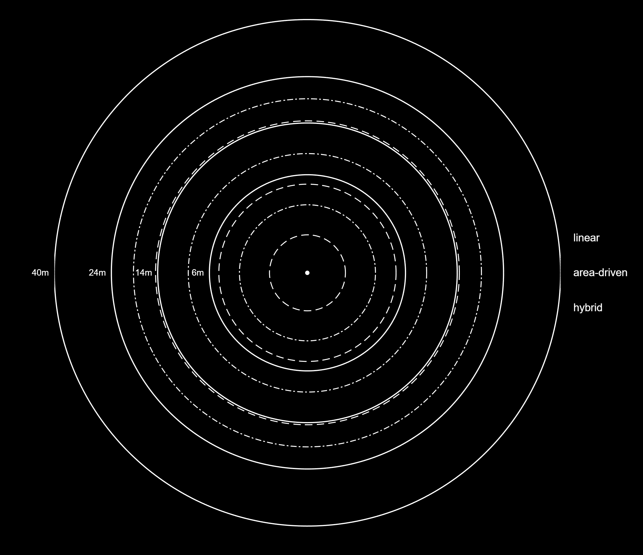
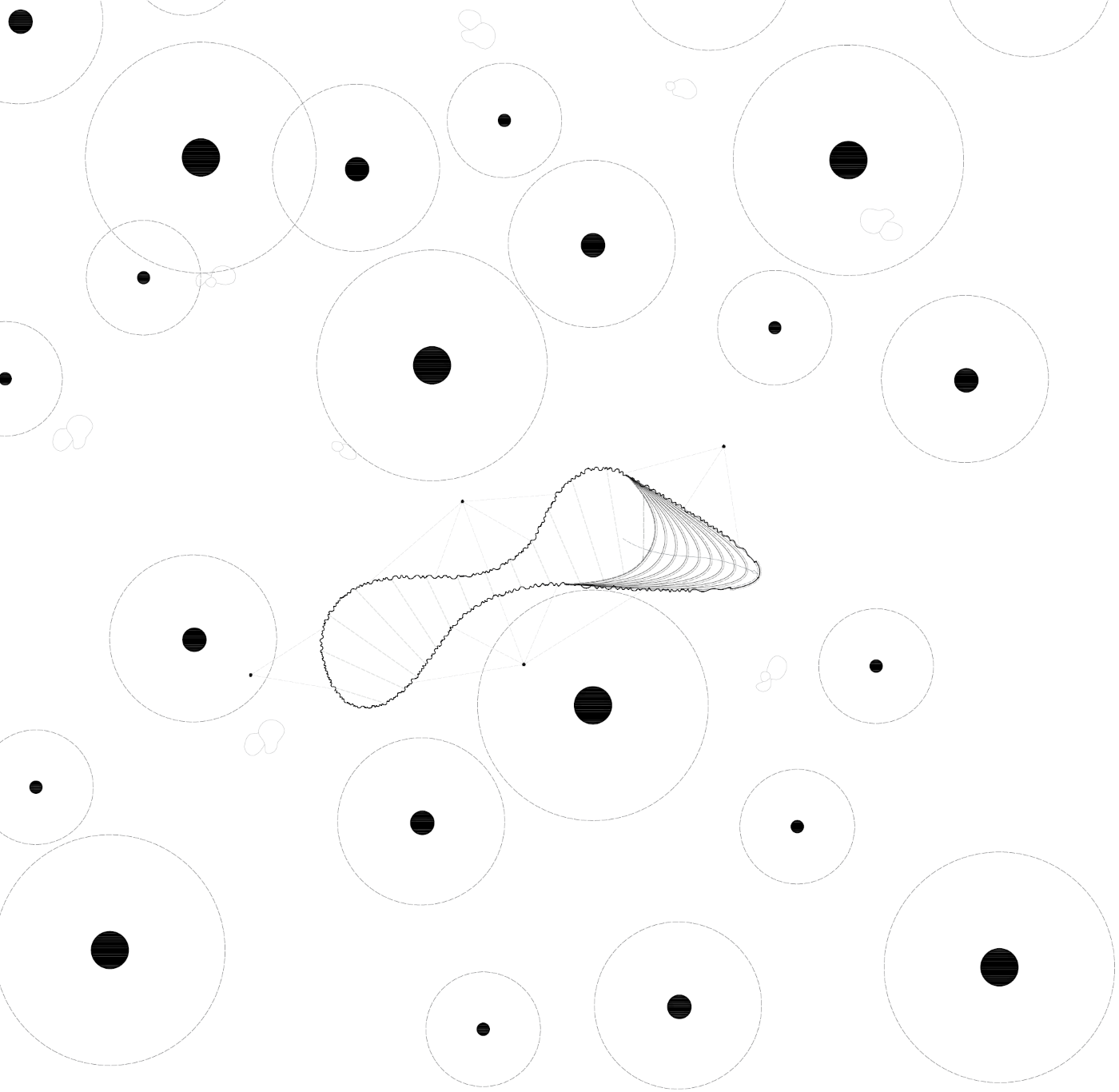
At this stage, the aim is not to define form too early, but to understand the relations that already structure the site. In Thinking the Forest and ILHA, code is used as a reading instrument: it helps register proximity, growth, fluctuation, and spatial pressure, so that the project can emerge from existing conditions rather than from a purely imposed image.

Open project
Thinking the Forest site reading image

Code, MATLAB

Root growth

max_radius = 16;
max_depth  = 8;
max_height = 40;
steps = [6 14 24 40];
max_incumbrance_planar = 0.5*pi*max_radius*max_depth;
% 1. Linear approximation
r_lin = max_radius .* steps ./ max_height;
% 2. Area-driven approximation
incumbrance_planar = max_incumbrance_planar .* steps ./ max_height;
r_area = sqrt(4*incumbrance_planar/pi);
% 3. Hybrid approximation
r_hyb = mean([r_lin; r_area],1);
theta = linspace(0,2*pi,500);
figure('Color','k','Position',[100 80 900 900])
hold on
axis equal
axis off
set(gca,'Color','k')
plot(0,0,'wo','MarkerFaceColor','w','MarkerSize',4)
for i = 1:length(steps)
    x_lin = r_lin(i)*cos(theta);
    y_lin = r_lin(i)*sin(theta);
    plot(x_lin,y_lin,'w--','LineWidth',1.0)
    x_area = r_area(i)*cos(theta);
    y_area = r_area(i)*sin(theta);
    plot(x_area,y_area,'w-','LineWidth',1.2)
    x_hyb = r_hyb(i)*cos(theta);
    y_hyb = r_hyb(i)*sin(theta);
    plot(x_hyb,y_hyb,'w-.','LineWidth',1.0)
end
for i = 1:length(steps)
    text(-r_area(i)-0.35,0,sprintf('%dm',steps(i)), ...
        'Color','w', ...
        'FontSize',9, ...
        'HorizontalAlignment','right', ...
        'VerticalAlignment','middle')
end
text(r_lin(end)+0.8,  2.2, 'linear', ...
    'Color','w','FontSize',11,'HorizontalAlignment','left')

text(r_area(end)+0.8, 0.0, 'area-driven', ...
    'Color','w','FontSize',11,'HorizontalAlignment','left')
text(r_hyb(end)+0.8, -2.2, 'hybrid', ...
    'Color','w','FontSize',11,'HorizontalAlignment','left')
title('Planimetric growth approximations', ...
      'Color','w', ...
      'FontSize',15, ...
      'FontWeight','bold')

Plot

Planimetric growth approximation

Plot

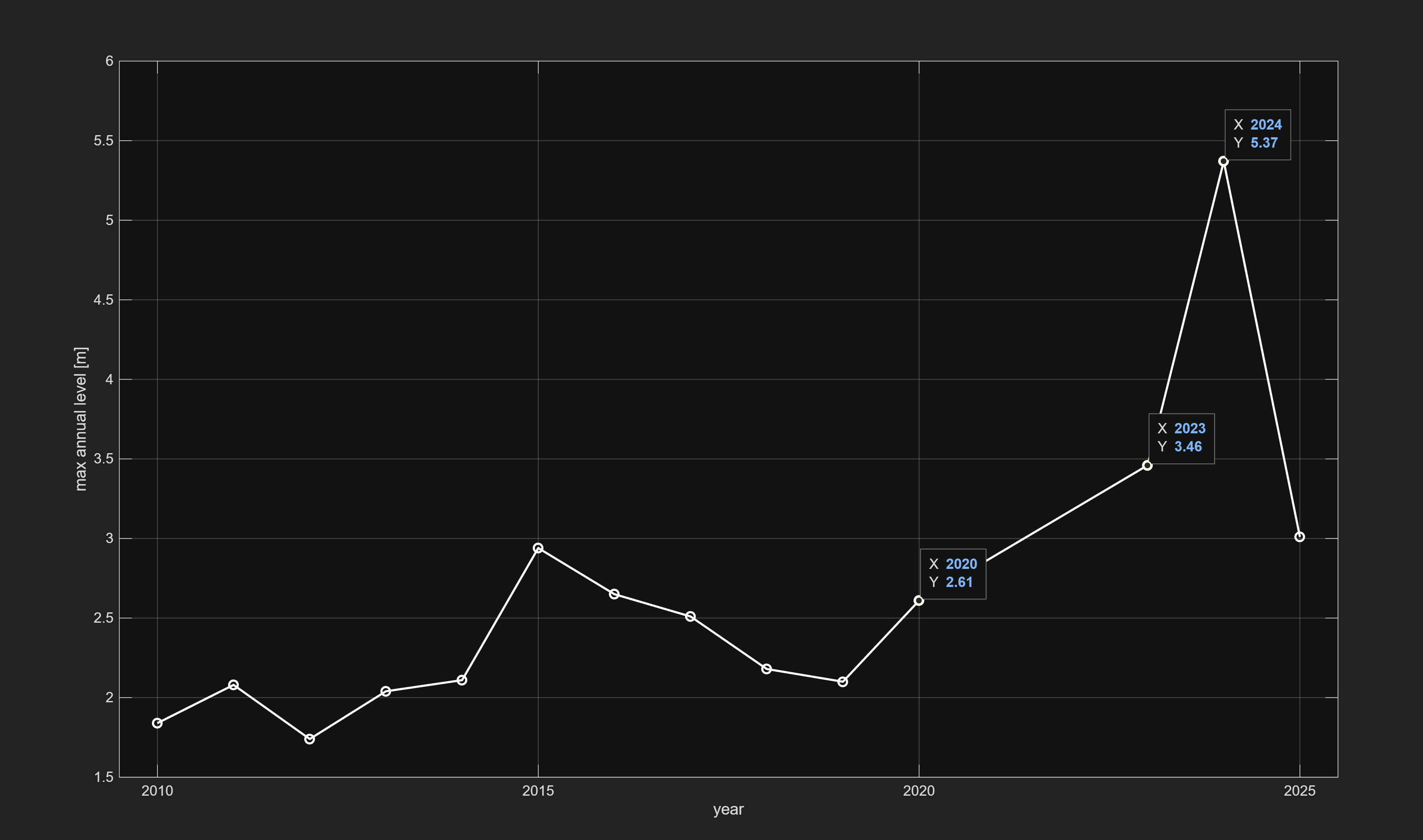
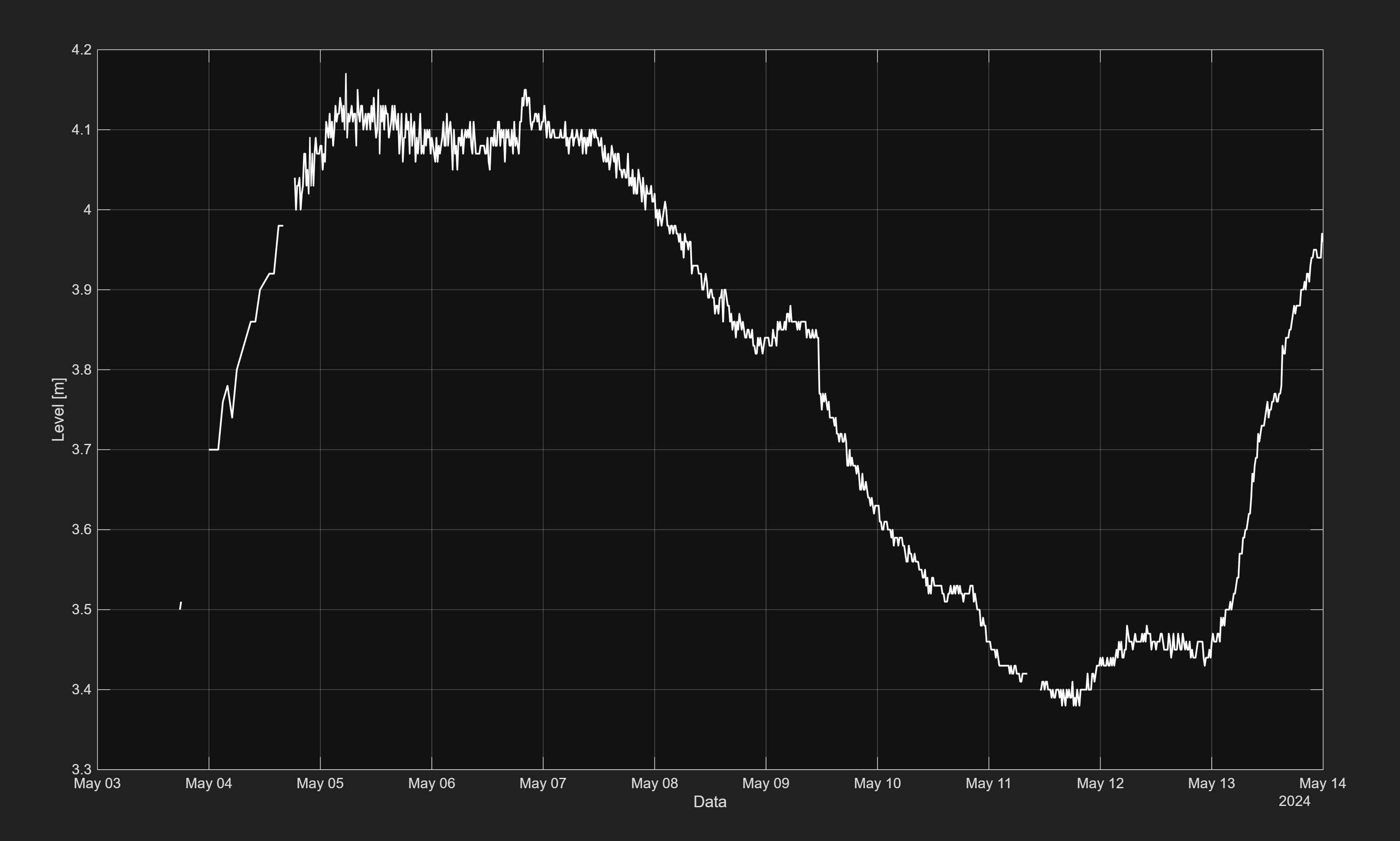
In ILHA, this reading phase focuses on environmental behaviour. Water levels are treated not as background data, but as an active condition shaping occupation, safety, and spatial decisions.

Open project

Code, MATLAB

Water level fluctuation

%% YEARS 2010-2025
years = 2010:2025;
hmax  = [1.84 2.08 1.74 2.04 2.11 2.94 2.65 2.51 2.18 2.10 ...
         2.61 NaN NaN 3.46 5.37 3.01];
valid = ~isnan(hmax);
figure;
plot(years(valid), hmax(valid), '-o', 'LineWidth', 1.5, 'MarkerSize', 6);
grid on;
xlabel('year');
ylabel('max annual level [m]');
title('Water level of Guaíba in Porto Alegre (2010–2025)');
xlim([2009.5 2025.5]);
ylim([1.5 6]);  

%% FROM MARCH TO MAY 2024
fname = '87450020-USINA DO GASOMETRO.txt';
fid = fopen(fname, 'r');
if fid == -1
    error('Impossibile aprire il file %s. Cartella corrente: %s', fname, pwd);
end
C = textscan(fid, '%s', 'Delimiter', '\n', 'Whitespace', '');
fclose(fid);
lines = C{1};
t = datetime.empty(0,1);  
nivel = nan(0,1);             
for i = 1:numel(lines)
    L = lines{i};
    m = regexp(L, '^(\d{2}/\d{2}/\d{4}\s+\d{2}:\d{2}:\d{2})(.*)', 'tokens', 'once');
    if isempty(m)
        continue
    end
    dt_str = m{1};
    rest   = m{2};
    nums = regexp(rest, '\d+(\.\d+)?', 'match');
    if isempty(nums)
        t(end+1,1)     = datetime(dt_str,'InputFormat','dd/MM/yyyy HH:mm:ss');
        nivel(end+1,1) = NaN;
        continue
    end
    lastVal = str2double(nums{end});
    if numel(nums) >= 2 || lastVal >= 50
        lvl_cm = lastVal;
    else
        lvl_cm = NaN;   
    end
    t(end+1,1)     = datetime(dt_str,'InputFormat','dd/MM/yyyy HH:mm:ss');
    nivel(end+1,1) = lvl_cm;
end
nivel_m = nivel / 100;

figure;
plot(t, nivel_m, 'LineWidth', 1.2);
grid on;
xlabel('Data');
ylabel('Level [m]');
title('Idrometric Level – Usina do Gasômetro (87450020)');
yl = [floor(min(nivel_m(~isnan(nivel_m)))*10)/10, ...
      ceil(max(nivel_m(~isnan(nivel_m)))*10)/10];
ylim(yl);

Plot

Water level of Guaíba, 2010–2025

Plot

Plot

Idrometric Level, Usina do Gasômetro

Plot

02

Design

The process begins by observing forces that are already present.

At this stage, the aim is not to define form too early, but to understand the relations that already structure the site. In Thinking the Forest and ILHA, code is used as a reading instrument: it helps register proximity, growth, fluctuation, and spatial pressure, so that the project can emerge from existing conditions rather than from a purely imposed image.

Open project

Algorithm, Grasshopper

Voronoi geometry

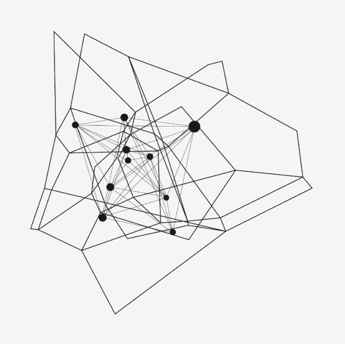
Voronoi geometry generated in Grasshopper

03

Test

Critical decisions are tested before being fully accepted.

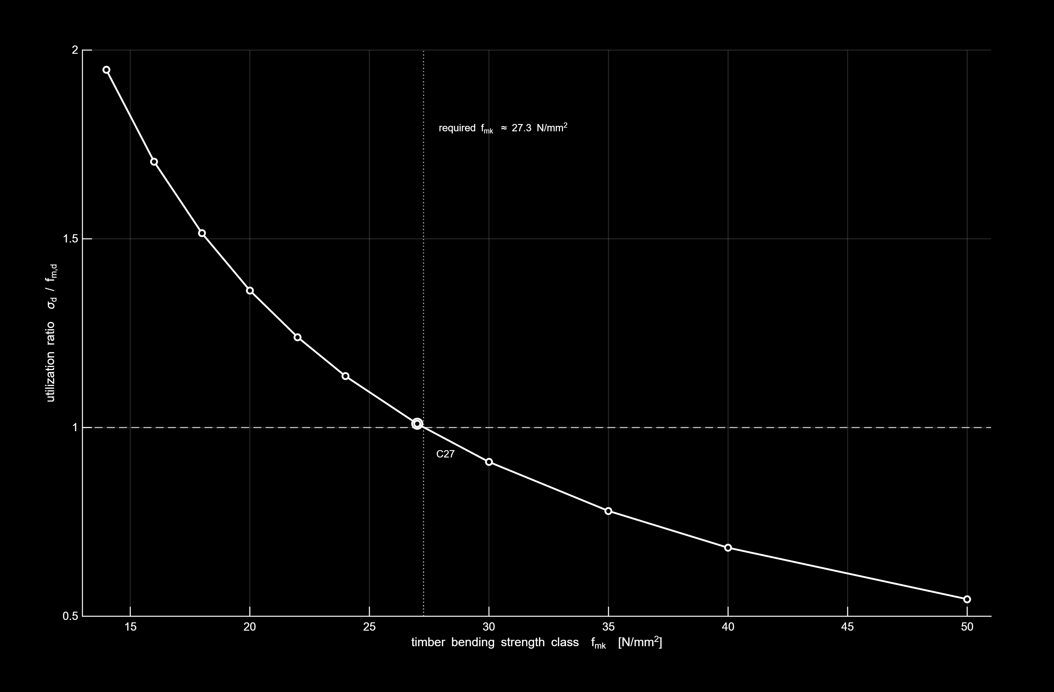
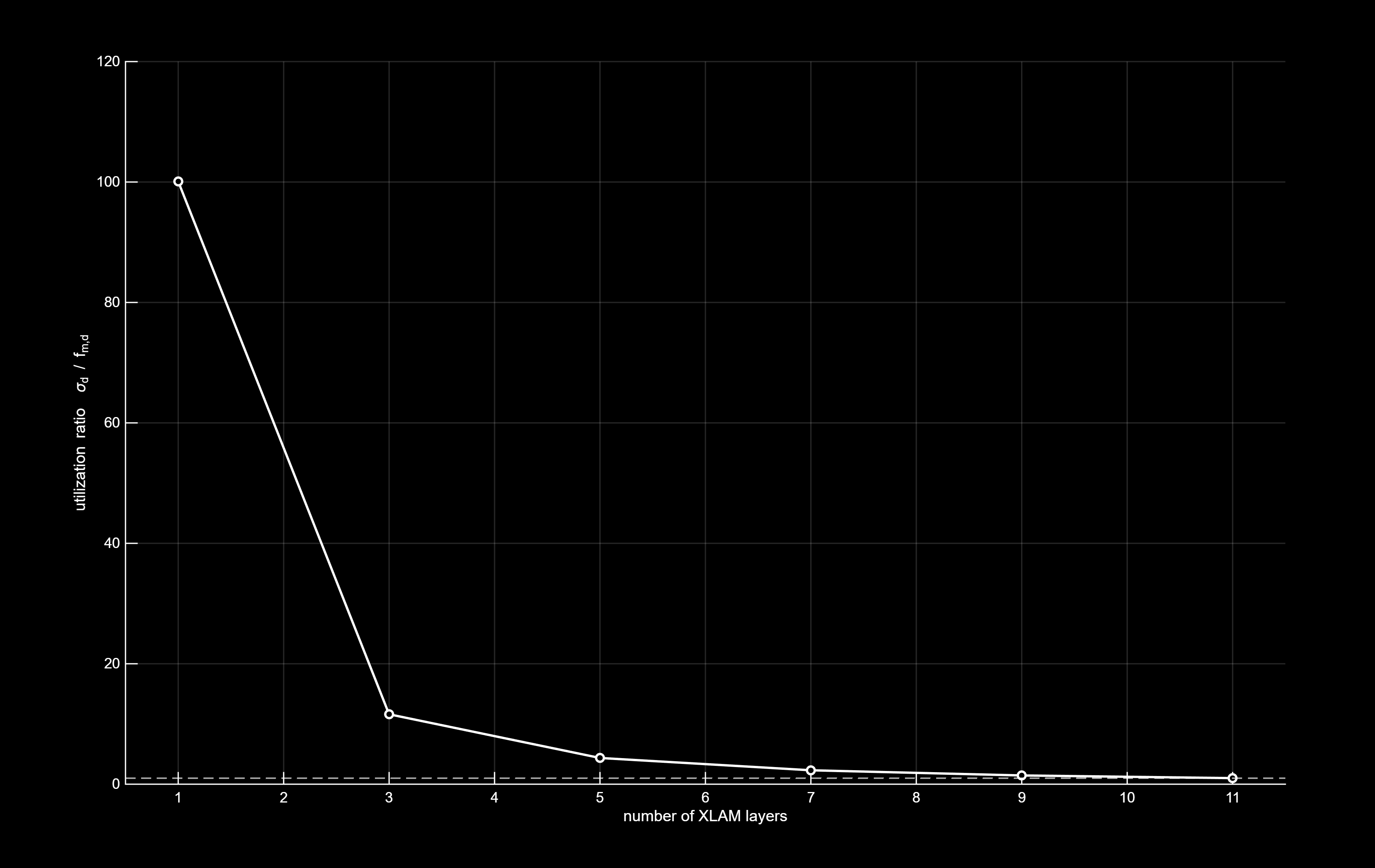
In Computational Tectonics, scripting becomes a way to verify whether a specific structural move can remain consistent with the architectural intention. The purpose is not simply to confirm a solution, but to understand its limits, measure its reliability, and identify where adjustment may still be necessary.

Open project
Computational Tectonics image

Code, MATLAB

Structural response check

a = 25.5;                     % [m]
b = 43;                       % [m]
Area_canopy = a * b;          % [m^2]
th_xlam_mono = 0.033;         % [m]
w_xlam_mono  = 0.158;         % [kN/m^2]
num_strati   = [1 3 5 7 9 11];
span = 16;                    % [m] structural span for strip verification
strip_width = 1;              % [m] unit strip
b_strip_mm = 1000;            % [mm] strip width
th_xlam_mono_mm = th_xlam_mono * 1000;  % [mm]
k_mod   = 0.8;
gamma_m = 1.45;
k_sys   = 1.1;
fm_k_ref = 27;                % [N/mm^2] reference timber class for plot 1 (C27)
% PERMANENT LOADS
q_s_concrete     = 1.00;      % [kN/m^2]
q_s_bracers      = 1.20;      % [kN/m^2]
q_s_hollowblocks = 0.56;      % [kN/m^2]
q_s_soletta      = q_s_concrete + q_s_bracers + q_s_hollowblocks;
% VARIABLE / ADDITIONAL LOADS
q_p_insulation = 0.10;        % [kN/m^2]
q_p_plaster    = 0.40;        % [kN/m^2]
q_p_floor      = q_p_insulation + q_p_plaster;
% TRUSS SYSTEM LOAD 
w_cpanel_s7 = 7 * w_xlam_mono;    % [kN/m^2]
n_truss_main = 19;
n_truss_sec  = 11;
sup_truss_sys_main = 2 * b * n_truss_main;   % [m^2]
sup_truss_sys_sec  = 2 * a * n_truss_sec;    % [m^2]
% scattered support patches / openings explicitly gathered
A_support_patches = 2 * (9.17 + 4.702*3 + 2.468*5 + 6.936*4);  % [m^2]
% simplified overlap correction at truss intersections
% assumes local overlap area proportional to panel thickness squared
n_s11 = 11;
th_cpanel_s11 = n_s11 * th_xlam_mono;        % [m]
A_intersections = 2 * (th_cpanel_s11^2) * n_truss_main * n_truss_sec;  % [m^2]
sup_truss_subtract = A_support_patches + A_intersections;      % [m^2]
sup_truss_sys = sup_truss_sys_main + sup_truss_sys_sec - sup_truss_subtract;
q_p_truss = sup_truss_sys / Area_canopy * w_cpanel_s7;         % [kN/m^2]
% SNOW LOAD
a_s  = 991;                                   % [m]
q_sk = 1.39 * (1 + (a_s / 728)^2);            % [kN/m^2]
mu_i = 0.8;
C_e  = 1.0;
C_t  = 1.0;
q_neve = q_sk * mu_i * C_e * C_t;             % [kN/m^2]
include_truss_in_panel_check = false;

coeff_layers = zeros(size(num_strati));
sigma_layers = zeros(size(num_strati));
q_ULS_layers = zeros(size(num_strati));
for idx = 1:length(num_strati)
    n_s = num_strati(idx);
    % self-weight of canopy for current build-up
    q_s_canopy = n_s * w_xlam_mono;                 % [kN/m^2]
    q_s = q_s_canopy + q_s_soletta;                 % [kN/m^2]
    % ULS load on the strip
    if include_truss_in_panel_check
        q_ULS = 1.3*q_s + 1.5*(q_p_floor + q_p_truss) + 1.5*q_neve;
    else
        q_ULS = 1.3*q_s + 1.5*q_p_floor + 1.5*q_neve;
    end
    q_ULS_layers(idx) = q_ULS;
    % convert area load to line load for a 1 m strip
    q_line = q_ULS * strip_width;                   % [kN/m]
    % maximum bending moment
    M_kNm = q_line * span^2 / 8;                    % [kN*m]
    M_Nmm = M_kNm * 1e6;                            % [N*mm]
    % homogenized rectangular section
    t_tot_mm = n_s * th_xlam_mono_mm;               % [mm]
    I_mm4 = b_strip_mm * t_tot_mm^3 / 12;           % [mm^4]
    y_mm  = t_tot_mm / 2;                           % [mm]
    % bending stress
    sigma = M_Nmm * y_mm / I_mm4;                   % [N/mm^2] = [MPa]
    sigma_layers(idx) = sigma;
    % design bending resistance
    f_m_d = k_sys * k_mod * fm_k_ref / gamma_m;     % [N/mm^2]
    % utilization ratio
    coeff_layers(idx) = sigma / f_m_d;
end
idx_ok = find(coeff_layers <= 1, 1, 'first');

fm_k_values = [14 16 18 20 22 24 27 30 35 40 50];
coeff_species = zeros(size(fm_k_values));
n_fix = 11;
q_s_canopy_fix = n_fix * w_xlam_mono;
q_s_fix = q_s_canopy_fix + q_s_soletta;

if include_truss_in_panel_check
    q_ULS_fix = 1.3*q_s_fix + 1.5*(q_p_floor + q_p_truss) + 1.5*q_neve;
else
    q_ULS_fix = 1.3*q_s_fix + 1.5*q_p_floor + 1.5*q_neve;
end
q_line_fix = q_ULS_fix * strip_width;              % [kN/m]
M_kNm_fix  = q_line_fix * span^2 / 8;              % [kN*m]
M_Nmm_fix  = M_kNm_fix * 1e6;                      % [N*mm]
t_fix_mm = n_fix * th_xlam_mono_mm;
I_fix_mm4 = b_strip_mm * t_fix_mm^3 / 12;
y_fix_mm  = t_fix_mm / 2;
sigma_fix = M_Nmm_fix * y_fix_mm / I_fix_mm4;      % [MPa]
for idx = 1:length(fm_k_values)
    fm_k = fm_k_values(idx);
    f_m_d = k_sys * k_mod * fm_k / gamma_m;
    coeff_species(idx) = sigma_fix / f_m_d;
end

fm_k_required = sigma_fix * gamma_m / (k_sys * k_mod);

figure('Color','k','Position',[80 80 900 700])
ax1 = axes;
hold(ax1,'on')
set(ax1,'Color','k', ...
    'XColor','w','YColor','w', ...
    'GridColor','w','GridAlpha',0.15, ...
    'FontName','Helvetica','FontSize',11, ...
    'LineWidth',1)
plot(num_strati, coeff_layers, 'w-o', ...
    'LineWidth',1.8, ...
    'MarkerSize',6, ...
    'MarkerFaceColor','k')
yline(1, 'w--', 'LineWidth',1.1)
if ~isempty(idx_ok)
    plot(num_strati(idx_ok), coeff_layers(idx_ok), ...
        'wo', 'MarkerSize',10, 'LineWidth',1.8)
    text(num_strati(idx_ok)+0.2, coeff_layers(idx_ok)-0.08, ...
        sprintf('first feasible: %d layers', num_strati(idx_ok)), ...
        'Color','w','FontSize',10)
end
xlabel('number of XLAM layers','Color','w')
ylabel('utilization ratio  \sigma_d / f_{m,d}','Color','w')
title('XLAM canopy: verification against panel build-up','Color','w','FontSize',14)
grid on
box off
xlim([min(num_strati)-0.5, max(num_strati)+0.5])

figure('Color','k','Position',[120 120 900 700])
ax2 = axes;
hold(ax2,'on')
set(ax2,'Color','k', ...
    'XColor','w','YColor','w', ...
    'GridColor','w','GridAlpha',0.15, ...
    'FontName','Helvetica','FontSize',11, ...
    'LineWidth',1)
plot(fm_k_values, coeff_species, 'w-o', ...
    'LineWidth',1.8, ...
    'MarkerSize',6, ...
    'MarkerFaceColor','k')
yline(1, 'w--', 'LineWidth',1.1)
idx_c27 = find(fm_k_values == 27, 1);
if ~isempty(idx_c27)
    plot(fm_k_values(idx_c27), coeff_species(idx_c27), ...
        'wo', 'MarkerSize',10, 'LineWidth',1.8)
    text(fm_k_values(idx_c27)+0.8, coeff_species(idx_c27)-0.08, ...
        'C27', 'Color','w', 'FontSize',10)
end
xline(fm_k_required, 'w:', 'LineWidth',1.1)
text(fm_k_required+0.6, max(coeff_species)*0.92, ...
    sprintf('required f_m_k \\approx %.1f N/mm^2', fm_k_required), ...
    'Color','w','FontSize',10)
xlabel('timber bending strength class  f_m_k  [N/mm^2]','Color','w')
ylabel('utilization ratio  \sigma_d / f_{m,d}','Color','w')
title('XLAM canopy: sensitivity to timber strength class','Color','w','FontSize',14)
grid on
box off
xlim([min(fm_k_values)-1, max(fm_k_values)+1])

Plot B

XLAM canopy: sensitivity to timber strength class

Plot

Plot A

XLAM canopy: verification against panel build-up

Plot

04

Activate

Performance is part of the architectural system.

With ILHA, the project is asked to do more than provide form. It is also developed as a system able to collect, filter, store, and support life under stressed conditions. At this stage, the reasoning shifts toward operational capacity: how much can be captured, produced, or sustained, and what degree of autonomy the architecture can realistically provide.

Open project
ILHA image one
ILHA image two
ILHA image three

Code, MATLAB

Rainwater collection and use

% Daily water demand per use [L/use]
Hands_Washing   = 2;
Shower          = 35;
Manual_Washing  = 15;
Washingmachine  = 60;
Flush           = 4;
% Daily workload [uses/day]
n_HandsWashing   = 500;
n_Shower         = 200;
n_ManualWashing  = 60;
n_Washingmachine = 30;
n_Flush          = 300;
% Daily demand [L/day]
WaterNeed_day = Hands_Washing*n_HandsWashing + ...
                Shower*n_Shower + ...
                Manual_Washing*n_ManualWashing + ...
                Washingmachine*n_Washingmachine + ...
                Flush*n_Flush;
WaterNeed_month = WaterNeed_day * 30;
fprintf('Total Average Workload Water Need Daily: %.2f L/day\n', WaterNeed_day);
fprintf('Total Average Workload Water Need Monthly: %.2f L/month\n', WaterNeed_month);
%% Collection surface
a = 21.42;      % [m]
b = 17.20;      % [m]
S = a*b;        % [m^2]
C_friction = 0.9;
loss = 0.05;
efficiency = C_friction * (1-loss);
%% Monthly rainfall [mm/month]
mm_rain = [144 135 117 116 109 116 136 121 150 174 132 130];
%% Monthly collected water [L/month]
Collection_month = mm_rain .* S .* efficiency;
Collection_max = max(Collection_month);
Collection_min = min(Collection_month);
fprintf('Maximum Collected Water: %.2f L/month\n', Collection_max);
fprintf('Minimum Collected Water: %.2f L/month\n', Collection_min);
percentageCovered_max = (Collection_max / WaterNeed_month) * 100;
percentageCovered_min = (Collection_min / WaterNeed_month) * 100;
fprintf('Maximum monthly coverage: %.2f%%\n', percentageCovered_max);
fprintf('Minimum monthly coverage: %.2f%%\n', percentageCovered_min);

Code, MATLAB

Energy production from relative motion

% RHD = regenerative hydraulic dampers
% TLCD = tuned liquid column damper integrated in pile
% All daily energies are expressed in kWh/day

%% Energy harvesting param
%RHD system
n_dampers      = 12;
deltaP_MPa     = 2;                 % [MPa]
deltaP_Pa      = deltaP_MPa * 1e6;  % [Pa]
d_piston       = 0.063;             % [m]
A_RHD          = pi * d_piston^2 / 4;   % [m^2]
f_RHD          = 0.2;               % [Hz]
Z_avg          = 0.10;              % [m]
Z_full         = 0.25;              % [m]
eff_chain_RHD  = 0.70;              % overall mech-elec efficiency
%TLCD-in-pile system
n_TLCD         = 2;
rho_water      = 1000;              % [kg/m^3]
g              = 9.81;              % [m/s^2]
eff_turb_ele   = 0.60;              % turbine + electric efficiency
D_TLCD         = 0.25;              % [m]
A_TLCD         = pi * D_TLCD^2 / 4; % [m^2]
f_TLCD         = 0.2;               % [Hz]
% Assumption: TLCD oscillation amplitude follows the same order of motion
Y_avg          = Z_avg;             % [m]
Y_full         = Z_full;            % [m]
% Duty / activation factor during the day
psi_avg        = 0.15;              % calm conditions
psi_full       = 0.50;              % flooding / energetic conditions

%% Istantaneous power
% RHD power [W]
P_RHD_avg_W  = 4 * n_dampers * deltaP_Pa * A_RHD  * f_RHD  * Z_avg  * eff_chain_RHD;
P_RHD_full_W = 4 * n_dampers * deltaP_Pa * A_RHD  * f_RHD  * Z_full * eff_chain_RHD;
% TLCD power [W]
P_TLCD_avg_W  = n_TLCD * (4 * rho_water * g * eff_turb_ele * A_TLCD * f_TLCD * Y_avg^2);
P_TLCD_full_W = n_TLCD * (4 * rho_water * g * eff_turb_ele * A_TLCD * f_TLCD * Y_full^2);


%% ENERGY PRODUCTION
Eday_RHD_avg_kWh   = (P_RHD_avg_W  / 1000) * 24 * psi_avg;
Eday_RHD_full_kWh  = (P_RHD_full_W / 1000) * 24 * psi_full;
Eday_TLCD_avg_kWh  = (P_TLCD_avg_W  / 1000) * 24 * psi_avg;
Eday_TLCD_full_kWh = (P_TLCD_full_W / 1000) * 24 * psi_full;
totalEnergy_avg_kWh  = Eday_RHD_avg_kWh  + Eday_TLCD_avg_kWh;
totalEnergy_full_kWh = Eday_RHD_full_kWh + Eday_TLCD_full_kWh;

%% ENERGY REQUIREMENT
% Water pumping
H_lift       = 5;       % [m] vertical head between tank base and filter
eff_pump     = 0.60;
V_water      = 14;      % [m^3/day]
E_pump_kWh   = rho_water * g * H_lift * V_water / (eff_pump * 3.6e6);
% UV filtration
P_UV_W       = 25;      % [W]
t_UV_h       = 12;      % [h/day]
E_UV_kWh     = P_UV_W * t_UV_h / 1000;
% Washing machines
E_WM_cycle_kWh = 0.5;   % [kWh/cycle]
n_WM_cycles    = 30;    % [cycles/day]
E_WM_kWh       = E_WM_cycle_kWh * n_WM_cycles;
% Lighting
LPD_W_m2     = 6;       % [W/m^2]
S_lit_m2     = 300;     % [m^2]
t_light_h    = 6;       % [h/day]
E_lights_kWh = LPD_W_m2 * S_lit_m2 * t_light_h / 1000;

totalEnergy_required_kWh = E_pump_kWh + E_UV_kWh + E_WM_kWh + E_lights_kWh;
coverage_avg_pct  = 100 * totalEnergy_avg_kWh  / totalEnergy_required_kWh;
coverage_full_pct = 100 * totalEnergy_full_kWh / totalEnergy_required_kWh;

fprintf('\n--- ENERGY PRODUCTION ---\n');
fprintf('Average conditions : Produced = %6.2f kWh/day\n', totalEnergy_avg_kWh);
fprintf('Flood conditions   : Produced = %6.2f kWh/day\n', totalEnergy_full_kWh);
fprintf('\n--- ENERGY DEMAND ---\n');
fprintf('Pump              = %6.2f kWh/day\n', E_pump_kWh);
fprintf('UV filter         = %6.2f kWh/day\n', E_UV_kWh);
fprintf('Washing machines  = %6.2f kWh/day\n', E_WM_kWh);
fprintf('Lighting          = %6.2f kWh/day\n', E_lights_kWh);
fprintf('Total required    = %6.2f kWh/day\n', totalEnergy_required_kWh);
fprintf('\n--- COVERAGE ---\n');
fprintf('Average conditions : %6.1f%%\n', coverage_avg_pct);
fprintf('Flood conditions   : %6.1f%%\n\n', coverage_full_pct);

Code, MATLAB

CO2 analysis [partial]

% Water pavilion structure
rho_steel = 7850;   % [kg/m^3]
% Poles
n_pole = 12;
D_pole = 0.8128;
d_pole = 0.7878;
L_pole = 13;
m_pole = n_pole * rho_steel * pi/4 * (D_pole^2 - d_pole^2) * L_pole;   % [kg]
% Rings
n_ring = 5;
D_ring = 12;
L_ring = pi * D_ring;
ms_HEB140 = 33.7;   % [kg/m]
m_ring = n_ring * ms_HEB140 * L_ring;   % [kg]
% Joints
n_joint = 60;
D_plate = 0.8128;
h_plate = 0.18;
sp_plate = 0.012;
v_joint = pi * D_plate * h_plate * sp_plate;   % [m^3] thin cylindrical approximation
m_gusset = 5;   % [kg/joint]
m_joint = n_joint * (v_joint * rho_steel + m_gusset);   % [kg]
% X-bracing
n_Xbracing = n_pole * (n_ring - 1) * 2;
L_brace = sqrt(2.5^2 + (D_ring * sin(pi/12))^2);
L_Xbracing = n_Xbracing * L_brace;
d_bracing = 0.016;
m_Xbracing = pi * d_bracing^2 / 4 * rho_steel * L_Xbracing;   % [kg]
% Bolts
n_bolts = 600;
m_bolt = 0.12;   % [kg]
m_bolts = n_bolts * m_bolt;   % [kg]
% Total steel mass
m_steel_tot_kg = m_pole + m_ring + m_Xbracing + m_joint + m_bolts;
m_steel_tot_t = m_steel_tot_kg / 1000;   % [t]

%% EMISSIONS
EF_steel_new     = 1.90;   % [tCO2 / t_steel]
EF_steel_EAF     = 0.70;   % recycled
EF_steel_reused  = 0.08;   % reused / reconditioned
emission_CO2_steel_new = m_steel_tot_t * EF_steel_new;
emission_CO2_steel_reused = m_steel_tot_t * EF_steel_reused;
EF_road  = 0.08;   % [kgCO2 / (t km)]
EF_barge = 0.03;   % [kgCO2 / (t km)]
km_road_RG   = 320;
km_barge_RG  = 10;
km_road_PA   = 5;
km_barge_PA  = 3;
CO2_transport_RG = (m_steel_tot_t * km_road_RG * EF_road + m_steel_tot_t * km_barge_RG * EF_barge) / 1000;   % [tCO2]
CO2_transport_PA = (m_steel_tot_t * km_road_PA * EF_road + m_steel_tot_t * km_barge_PA * EF_barge) / 1000;   % [tCO2]
CO2_total_RG_new    = emission_CO2_steel_new    + CO2_transport_RG;
CO2_total_PA_new    = emission_CO2_steel_new    + CO2_transport_PA;
CO2_total_RG_reused = emission_CO2_steel_reused + CO2_transport_RG;
CO2_total_PA_reused = emission_CO2_steel_reused + CO2_transport_PA;

fprintf('Rio Grande   | all new  : %8.3f tCO2\n', CO2_total_RG_new);
fprintf('Porto Alegre | all new  : %8.3f tCO2\n', CO2_total_PA_new);
fprintf('Rio Grande   | reused   : %8.3f tCO2\n', CO2_total_RG_reused);
fprintf('Porto Alegre | reused   : %8.3f tCO2\n', CO2_total_PA_reused);
RainwaterMaximum monthly coverage : 15.35%
Minimum monthly coverage : 9.62%
Energy coverageAverage conditions : 57.2%
Flood conditions : 477.1%
AutonomyRio Grande | all new : 93.238 tCO2
Porto Alegre | all new : 92.008 tCO2
Rio Grande | reused : 5.127 tCO2
Porto Alegre | reused : 3.897 tCO2

05

Respond

The final step considers how architecture may adjust over time.

In Designing Habitability, physiological conditions are translated into luminous output so that atmosphere and use can vary in relation to changing states. Here code is no longer only analytical or verificatory; it begins to participate in the behaviour of the space itself, allowing the project to respond rather than remain entirely fixed.

Open project

, ARDUINO

Physio-light mapping

#include WiFi.h
#include WebServer.h
#include Adafruit_NeoPixel.h
#include stdio.h
#include string.h
#include ctype.h
#define LED_PIN        18
#define NUM_LEDS       58
#define MAX_ROWS       100
#define STEP_TIME_MS   3000UL

const char* AP_SSID = "PHYSIO_LIGHT_DEMO";
const char* AP_PASSWORD = "physiolight";
Adafruit_NeoPixel strip(NUM_LEDS, LED_PIN, NEO_GRB + NEO_KHZ800);
WebServer server(80);
const char csvData[] =
"r,g,b,brightness\n"
"255,130,0,6\n"
"255,130,0,6\n"
"255,130,0,6\n"
"255,131,0,6\n"
"255,137,15,7\n"
"255,140,24,7\n"
"255,143,31,7\n"
"255,164,82,8\n"
"255,168,91,9\n"
"255,174,102,11\n"
"255,178,111,12\n"
"255,183,122,13\n"
"255,185,127,15\n"
"255,187,130,16\n"
"255,189,134,16\n"
"255,190,135,17\n"
"255,192,139,18\n"
"255,193,141,21\n"
"255,194,143,196\n"
"255,195,145,210\n"
"255,196,147,213\n"
"255,197,150,216\n"
"255,198,151,218\n"
"255,200,155,220\n"
"255,202,158,221\n"
"255,203,160,223\n"
"255,204,162,224\n"
"255,207,168,225\n"
"255,209,172,225\n"
"255,211,175,226\n"
"255,213,180,228\n"
"255,217,187,228\n"
"255,223,197,230\n"
"255,228,205,231\n"
"255,229,208,233\n"
"255,232,212,234\n"
"255,234,217,234\n"
"255,236,220,235\n"
"255,237,221,237\n"
"255,240,226,237\n"
"255,249,241,237\n"
"255,250,244,239\n"
"255,251,245,240\n"
"255,251,245,240\n"
"255,251,245,240\n"
"255,250,244,239\n"
"255,249,241,237\n"
"255,240,226,237\n"
"255,237,221,237\n"
"255,236,220,235\n"
"255,234,217,234\n"
"255,232,212,234\n"
"255,229,208,233\n"
"255,228,205,231\n"
"255,223,197,230\n"
"255,217,187,228\n"
"255,213,180,228\n"
"255,211,175,226\n"
"255,209,172,225\n"
"255,207,168,225\n"
"255,204,162,224\n"
"255,203,160,223\n"
"255,202,158,221\n"
"255,200,155,220\n"
"255,198,151,218\n"
"255,197,150,216\n"
"255,196,147,213\n"
"255,195,145,210\n"
"255,194,143,196\n"
"255,193,141,21\n"
"255,192,139,18\n"
"255,190,135,17\n"
"255,189,134,16\n"
"255,187,130,16\n"
"255,185,127,15\n"
"255,183,122,13\n"
"255,178,111,12\n"
"255,174,102,11\n"
"255,168,91,9\n"
"255,164,82,8\n"
"255,143,31,7\n"
"255,140,24,7\n"
"255,137,15,7\n"
"255,131,0,6\n"
"255,130,0,6\n"
"255,130,0,6\n"
"255,130,0,6\n";

struct LedStep {  uint8_t r;  uint8_t g;  uint8_t b;  uint8_t brightness;};
LedStep steps[MAX_ROWS];
int stepCount = 0;
int currentStep = 0;
unsigned long lastStepChange = 0;
bool simulationRunning = false;
uint8_t manualR = 255;
uint8_t manualG = 160;
uint8_t manualB = 90;
uint8_t manualBrightness = 40;
String manualState = "manual";
String manualMode = "manual";
uint8_t clampToByte(int value) {  if (value < 0) return 0;  if (value > 255) return 255;  return (uint8_t)value;}
void addCorsHeaders() {  server.sendHeader("Access-Control-Allow-Origin", "*");  server.sendHeader("Access-Control-Allow-Headers", "Content-Type");
  server.sendHeader("Access-Control-Allow-Methods", "GET,POST,OPTIONS");}
void sendJsonResponse(int code, const String& payload) {  addCorsHeaders();  server.send(code, "application/json", payload);}
void handleOptions() {  addCorsHeaders();  server.send(204);}
bool extractIntField(const String& body, const char* key, int& valueOut) {
  int keyPos = body.indexOf(key);
  if (keyPos < 0) return false;
  int colonPos = body.indexOf(':', keyPos);
  if (colonPos < 0) return false;
  int pos = colonPos + 1;
  while (pos < body.length() && isspace((unsigned char)body[pos])) pos++;
  bool negative = false;
  if (pos < body.length() && body[pos] == '-') {
    negative = true;
    pos++;
  }
  int start = pos;
  while (pos < body.length() && isdigit((unsigned char)body[pos])) pos++;
  if (start == pos) return false;
  int parsed = body.substring(start, pos).toInt();
  valueOut = negative ? -parsed : parsed;
  return true;
}

String extractStringField(const String& body, const char* key) {
  int keyPos = body.indexOf(key);
  if (keyPos < 0) return "";
  int colonPos = body.indexOf(':', keyPos);
  if (colonPos < 0) return "";
  int firstQuote = body.indexOf('"', colonPos + 1);
  if (firstQuote < 0) return "";
  int secondQuote = body.indexOf('"', firstQuote + 1);
  if (secondQuote < 0) return "";
  return body.substring(firstQuote + 1, secondQuote);
}
void applyColorToStrip(uint8_t r, uint8_t g, uint8_t b, uint8_t brightness) {
  uint8_t rScaled = (uint16_t)r * brightness / 255;
  uint8_t gScaled = (uint16_t)g * brightness / 255;
  uint8_t bScaled = (uint16_t)b * brightness / 255;
  for (int i = 0; i < NUM_LEDS; i++) {
    strip.setPixelColor(i, strip.Color(rScaled, gScaled, bScaled));
  }
  strip.show();
}
void showSimulationStep(int index) {
  if (index < 0 || index >= stepCount) return;
  applyColorToStrip(
    steps[index].r,
    steps[index].g,
    steps[index].b,
    steps[index].brightness
  );
  Serial.print("SIM step ");
  Serial.print(index + 1);
  Serial.print("/");
  Serial.print(stepCount);
  Serial.print(" -> RGB(");
  Serial.print(steps[index].r);
  Serial.print(", ");
  Serial.print(steps[index].g);
  Serial.print(", ");
  Serial.print(steps[index].b);
  Serial.print(") BR ");
  Serial.println(steps[index].brightness);
}
void showManualScene() {
  applyColorToStrip(manualR, manualG, manualB, manualBrightness);
  Serial.print("MANUAL -> RGB(");
  Serial.print(manualR);
  Serial.print(", ");
  Serial.print(manualG);
  Serial.print(", ");
  Serial.print(manualB);
  Serial.print(") BR ");
  Serial.print(manualBrightness);
  Serial.print(" | state: ");
  Serial.print(manualState);
  Serial.print(" | mode: ");
  Serial.println(manualMode);
}
void parseCSV() {
  stepCount = 0;
  char buffer[sizeof(csvData)];
  strncpy(buffer, csvData, sizeof(buffer) - 1);
  buffer[sizeof(buffer) - 1] = '\0';
  char* line = strtok(buffer, "\n");
  bool firstLine = true;
  while (line != NULL && stepCount < MAX_ROWS) {
    if (firstLine) {
      firstLine = false;
    } else {
      int r, g, b, brightness;
      int parsed = sscanf(line, "%d,%d,%d,%d", &r, &g, &b, &brightness);
      if (parsed == 4) {
        steps[stepCount].r = clampToByte(r);
        steps[stepCount].g = clampToByte(g);
        steps[stepCount].b = clampToByte(b);
        steps[stepCount].brightness = clampToByte(brightness);
        stepCount++;
      }
    }
    line = strtok(NULL, "\n");
  }
}
void handleRoot() {
  String html =
    "Physio Light ESP32"
    "

Physio Light ESP32 is online

" "

POST /light

" "

POST /simulation/start

" "

POST /simulation/stop

" "

GET /status

" ""; addCorsHeaders(); server.send(200, "text/html", html); } void handleStatus() { String mode = simulationRunning ? "simulation" : "manual"; String json = "{"; json += "\"ok\":true,"; json += "\"mode\":\"" + mode + "\","; json += "\"simulation_running\":" + String(simulationRunning ? "true" : "false") + ","; json += "\"current_step\":" + String(currentStep) + ","; json += "\"step_count\":" + String(stepCount) + ","; json += "\"step_time_ms\":" + String(STEP_TIME_MS) + ","; json += "\"ip\":\"" + WiFi.softAPIP().toString() + "\""; json += "}"; sendJsonResponse(200, json); } void handleLight() { if (!server.hasArg("plain")) { sendJsonResponse(400, "{\"ok\":false,\"error\":\"Missing JSON body\"}"); return; } String body = server.arg("plain"); int r = manualR; int g = manualG; int b = manualB; int brightness = manualBrightness; if (!extractIntField(body, "\"r\"", r) || !extractIntField(body, "\"g\"", g) || !extractIntField(body, "\"b\"", b) || !extractIntField(body, "\"brightness\"", brightness)) { sendJsonResponse(400, "{\"ok\":false,\"error\":\"JSON must contain r, g, b, brightness\"}"); return; } manualR = clampToByte(r); manualG = clampToByte(g); manualB = clampToByte(b); manualBrightness = clampToByte(brightness); String parsedState = extractStringField(body, "\"state\""); String parsedMode = extractStringField(body, "\"mode\""); if (parsedState.length() > 0) manualState = parsedState; if (parsedMode.length() > 0) manualMode = parsedMode; simulationRunning = false; showManualScene(); String json = "{"; json += "\"ok\":true,"; json += "\"mode\":\"manual\","; json += "\"r\":" + String(manualR) + ","; json += "\"g\":" + String(manualG) + ","; json += "\"b\":" + String(manualB) + ","; json += "\"brightness\":" + String(manualBrightness); json += "}"; sendJsonResponse(200, json); } void handleSimulationStart() { if (stepCount == 0) { sendJsonResponse(500, "{\"ok\":false,\"error\":\"No simulation steps loaded\"}"); return;} currentStep = 0; simulationRunning = true; lastStepChange = millis(); showSimulationStep(currentStep); String json = "{"; json += "\"ok\":true,"; json += "\"mode\":\"simulation\","; json += "\"step_count\":" + String(stepCount) + ","; json += "\"step_time_ms\":" + String(STEP_TIME_MS); json += "}"; sendJsonResponse(200, json); } void handleSimulationStop() { simulationRunning = false; showManualScene(); sendJsonResponse(200, "{\"ok\":true,\"mode\":\"manual\",\"simulation_running\":false}"); } void handleNotFound() { if (server.method() == HTTP_OPTIONS) { handleOptions(); return; } sendJsonResponse(404, "{\"ok\":false,\"error\":\"Not found\"}"); } void registerRoutes() { server.on("/", HTTP_GET, handleRoot); server.on("/status", HTTP_GET, handleStatus); server.on("/light", HTTP_POST, handleLight); server.on("/simulation/start", HTTP_POST, handleSimulationStart); server.on("/simulation/stop", HTTP_POST, handleSimulationStop); server.on("/light", HTTP_OPTIONS, handleOptions); server.on("/simulation/start", HTTP_OPTIONS, handleOptions); server.on("/simulation/stop", HTTP_OPTIONS, handleOptions); server.on("/status", HTTP_OPTIONS, handleOptions); server.onNotFound(handleNotFound); } void setupAccessPoint() { WiFi.mode(WIFI_AP); bool apStarted = WiFi.softAP(AP_SSID, AP_PASSWORD); Serial.println(); Serial.println("Wi-Fi Access Point"); Serial.print("SSID: "); Serial.println(AP_SSID); Serial.print("Password: "); Serial.println(AP_PASSWORD); Serial.print("Started: "); Serial.println(apStarted ? "yes" : "no"); Serial.print("IP: "); Serial.println(WiFi.softAPIP()); } void setup() { Serial.begin(115200); delay(1200); Serial.println(); Serial.println("PHYSIO LIGHT DEMO STARTING"); strip.begin(); strip.clear(); strip.show(); parseCSV(); Serial.print("Simulation steps loaded: "); Serial.println(stepCount); Serial.print("Total loop duration (s): "); Serial.println((stepCount * STEP_TIME_MS) / 1000.0f); setupAccessPoint(); registerRoutes(); server.begin(); Serial.println("HTTP server started"); showManualScene(); } void loop() { server.handleClient(); if (simulationRunning && stepCount > 0) { unsigned long now = millis(); if (now - lastStepChange >= STEP_TIME_MS) { currentStep++; if (currentStep >= stepCount) currentStep = 0; showSimulationStep(currentStep); lastStepChange = now; } } }
Live interface

Simplified version of the developed interface. Visit the PhysioApp interface to see more.

RGB 224 / 122 / 78 Brightness 61% Mode: Sleep